MODEL FITS

We have demonstrated scaling in our lattice data over the entire range of q² considered, and will now proceed with model fits. The following functional forms have been considered:

Gribov[3]

   

$${\frac{q^2}{q^4+M_{\scriptscriptstyle\rm IR}^4}}$$ (5)

Stingl[4]

 

$${\frac{q^2}{q^4+2A^2q^2+M_{\scriptscriptstyle\rm IR}^4}}$$ (6)

Marenzoni[5]

 

$${\frac{1}{(q^2)^{1+\alpha}+M_{\scriptscriptstyle\rm IR}^2}}$$ (7)

Cornwall[6]

 

$$\left[\vphantom{(q^2+M^2(q^2))\ln\frac{q^2+4M^2(q^2)}{\Lambda^2}}\right. {\frac{q^2+4M^2(q^2)}{\Lambda^2}} \left.\vphantom{(q^2+M^2(q^2))\ln\frac{q^2+4M^2(q^2)}{\Lambda^2}}\right]^{-1}_{}$$ (8)

Model A

 

$${\frac{A}{(q^2+M_{\scriptscriptstyle\rm IR}^2)^{1+\alpha}}}$$ (9)

Model B

 

$${\frac{A}{(q^2)^{1+\alpha}+(M_{\scriptscriptstyle\rm IR}^2)^{1+\alpha}}}$$ (10)

Model C

  

$$\alpha$$ (11)

where D(q²) $\equiv$ ZD_r(q²) and

 

$${\frac{1}{q^2+M_{\scriptscriptstyle\rm UV}^2}}$$ (12)

 

$$\left(\vphantom{\frac{1}{2}\ln((q^2+M^2)/M^2)}\right. {\textstyle\frac{1}{2}} \left.\vphantom{\frac{1}{2}\ln((q^2+M^2)/M^2)}\right)^{-d_D}_{}$$ (13)

$$\left\{\vphantom{\ln\frac{q^2+4M^2}{\Lambda^2}/ \ln\frac{4M^2}{\Lambda^2}}\right. {\frac{q^2+4M^2}{\Lambda^2}} {\frac{4M^2}{\Lambda^2}} \left.\vphantom{\ln\frac{q^2+4M^2}{\Lambda^2}/ \ln\frac{4M^2}{\Lambda^2}}\right\}^{-6/11}_{}$$

We have also considered the models A and B, which are constructed from models A and B by setting M_UV = M_IR. Gribov's and Stingl's models (5) and (6) are modified in order to exhibit the asymptotic behaviour of (2). Models A and B are constructed as generalisations of (7) with the correct dimension and asymptotic behaviour.

All models are fitted to the large lattice data using the cylindrical cut defined in [1,7]. The lowest momentum value was excluded, as the volume dependence of this point could not be assessed. In order to balance the sensitivity of the fit between the high- and low-momentum region, nearby data points within $\Delta$(qa) < 0.05 were averaged.

The $\chi^{2}_{}$ per degree of freedom and parameter values for fits to all these models are shown in table 1. It is clear that model B accounts for the data better than any of the other models. The best fit to this model is illustrated in fig. 2.

  

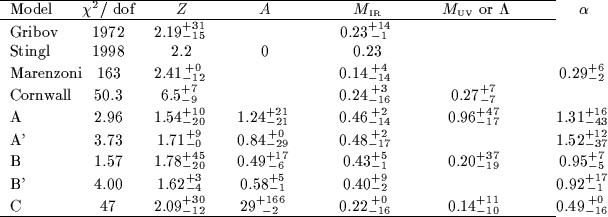
Table: Parameter values for fits to models (5)-(11). The values quoted are for fits to the entire set of data. The errors denote the uncertainties in the last digit(s) of the parameter values which result from varying the fitting range [8].

  

Figure: The gluon propagator multiplied by q², with nearby points averaged. The line illustrates our best fit to the form defined in (10). The scale is taken from the string tension [2].